From Measurement to Management: Integrating Cyberrisk Quantification into Risk Governance

The inclusion of the governance domain was arguably the most notable addition to the US National Institute of Standards and Technology (NIST) Cybersecurity Framework (CSF) 2.0, released in 2024.¹ This is meant to help provide consistent and repeated feedback loops to the rest of the NIST domains to ensure proper cybersecurity operations. Risk communication processes are thus improved as managers have tools to inform executives and boards and communicate with practitioners about what objectives to work on next.

One subcategory in the new governance category concerns the setting and management of risk appetite and tolerance. This is codified in GV.RM-02:

“Risk appetite and risk tolerance statements are established, communicated, and maintained.”² In its implementation guide, NIST offers these additional tasks to assist with putting this into practice:³

1. Determine and communicate risk appetite statements that convey expectations about the appropriate level of risk for the organization.
2. Translate risk appetite statements into specific, measurable, and broadly understandable risk tolerance statements.
3. Refine organizational objectives and risk appetite periodically based on known risk exposure and residual risk.

These tasks can be challenging for organizations to accomplish; however, cyberrisk quantification (CRQ) can be a key enabler.⁴ But even with a mature CRQ program, there is a need for techniques to help interpret the CRQ results and accomplish the aforementioned tasks.

It is worth deconstructing the requirements to operationalize risk governance, a distinct subset of tasks in a broader cybersecurity governance program. For the cyberrisk department and its partners in second-line risk functions (i.e., operational risk) there is a key list of tasks enabled by quantitatively led cyberrisk governance. These tasks are:

1. Setting a security budget
2. Selecting the parameters of cyberinsurance
3. Determining a plan for absorbing the financial impacts of cyberincidents on the firm’s balance sheet

There are several interrelated prerequisites to these tasks. Accomplishing these risk governance tasks will enable an organization to demonstrate compliance with the risk management subcategory.

Cyberrisk Governance Life Cycle

The processes mentioned account for the tasks involved in governing cyberrisk quantitatively (figure 1).

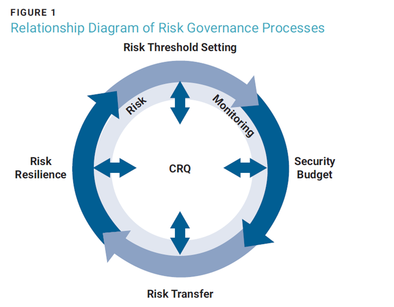
The process begins with a CRQ assessment and a selection of risk appetite values. Next, the organization identifies the amount of cybersecurity spending that needs to be allocated. Then an enterprise’s cyberinsurance policy can be optimized to account for appetite and coverage windows. Finally, the residual risk should be accounted for in a capital program. Throughout these steps, there are opportunities for organizations to revisit previous steps and revalidate their commitment to an appetite level (i.e., risk monitoring). If there is a disagreement about budget, coverage, or allocation at any of these steps, the organization should revalidate its feelings about the selected risk appetite value and adjust accordingly. Using this framework will allow organizations to operationalize risk governance and show adherence to the new NIST CSF 2.0 guidelines for risk appetite management in the governance domain.

Prerequisite 1: CRQ Assessments

A prerequisite to quantitative cyberrisk governance is the quantitative assessment of an enterprise’s risk profile. There are a variety of approaches to performing the assessment, but at its core, it will require the assessment of key risk scenarios and the creation of a corresponding list of probabilities and severity.⁵ Sometimes this is expressed in frequency and magnitude of loss, but these are all variations of the classic risk equation of probability and impact. A CRQ assessment can be done using data from subject matter expert (SME)-calibrated estimates or derived from large data sets and filtered for applicability to an organization.⁶ These values are then simulated using the Monte Carlo method to model future outcomes. ⁷ The product is a list of things that could go wrong, how likely they are to occur, and how much it would cost the organization if it were to happen. Assessing cyberrisk quantitatively has a sufficient body of work behind it, the coverage of which is out of the scope of this discussion.⁸ However, it is sufficient to identify here that it is relatively straightforward to accomplish and generates useful results for risk governance.

CRQ results are typically displayed graphically on a curve, sometimes called a loss exceedance curve (LEC) or an exceedance probability (EP) curve (figure 2). These curves show the probability that an organization will experience a loss at or above that point on the curve. Each curve is scoped by time (typically one year) and scenario.

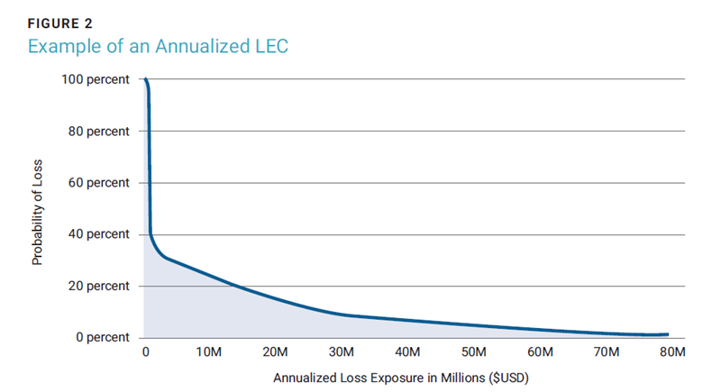
There are two general methods of expressing these curves: single loss expectancy (SLE) or annualized loss expectancy (ALE). Each has a different use case and implications for governance. Since these events are unlikely to happen yearly, it is important to express these losses in a way that accounts for their frequency. Annualizing the results is the typical way quantified cyberrisk is displayed. ALE shows the amount of risk that a firm has each year, effectively spreading the losses over the intervening years between now and when the event is expected to occur. Computing ALE is done by multiplying the loss amount of the event by the frequency of its occurrence. Assuming an event does not happen every year, it will result in a number that is less than the losses expected from any one occurrence of that event. The SLE value is the amount of the loss absent any modifications for frequency.

Usually, various points are taken from this curve to drive special actions. For example, the minimum (99%) and maximum (1%) values provide a complete range of losses. Other useful metrics to take from this are the average or most likely values (e.g., mode). A mode value provides a sense of a midpoint value for what a typical loss looks like. Generally, using the midpoint and max values drives better security hygiene than the minimum value. These metrics are helpful for governance by giving an organization a sense of what could happen and are a precursor to evaluating an organization’s balance sheet to see what the impact of a cyberincident would look like.

Prerequisite 2: Setting Risk Appetite/Materiality

The enabling task for proper risk governance is determining how much risk is acceptable. As important as it is to use quantified methods to accomplish this, determining how much is acceptable will largely be based on the stakeholder’s emotional response to a threshold.⁹ One way to accomplish this is to leverage a determination of materiality. In other words, any cyberevent that would be considered material would be unacceptable, and therefore it becomes a de facto risk appetite threshold.¹⁰

Determination of material cyberevents is a complex endeavor, however, frameworks exist to facilitate this process.¹¹ Finding these values involves using an enterprise’s revenue as a financial benchmark to compute a threshold based on it. Typically, financial materiality thresholds span from 4%-10%.¹² However, the threshold should likely be much lower for cybersecurity incidents, as much as 0.01% or one basis point (bps) of revenue.¹³ Taking a variety of thresholds from one to 100 basis points is key to selecting a materiality threshold. Suggesting a variety of thresholds is the same approach as getting decision makers to determine their appetite for risk—and basing it on materiality is a meaningful way to begin that conversation.

An example of a tool for threshold selection is a simple chart that displays precalculated thresholds based on the basis points of revenue (figure 3). One can select the probability of experiencing losses at those amounts from the loss exceedance curve. This enhances the threshold selection process by asking how much the enterprise is comfortable losing and what is the likelihood of experiencing losses at those amounts.

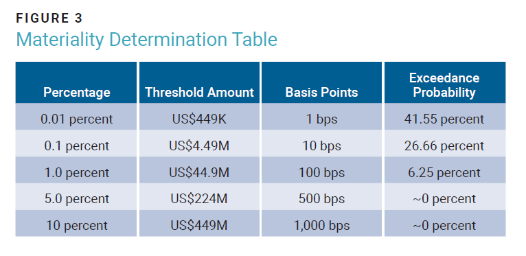
This table was established using an example organization’s revenue as of its last annual report, which was US$4.49 billion. That value was then multiplied by the basis point percentages to arrive at a threshold amount. The corresponding probability is taken at the intersection of the threshold amount on the LEC. The probability of exceeding the threshold helps provide another dimension to the selection process.

Selecting one of these values requires finding a threshold that is acceptable to all stakeholders. It is helpful to identify these proposed values as drafts and continue to refer to the chosen value as such until it is evaluated during the rest of the governance processes. Since something must be material, the options from the table at 500 and 1,000 bps are not reasonable.¹⁴

Cybersecurity Spending

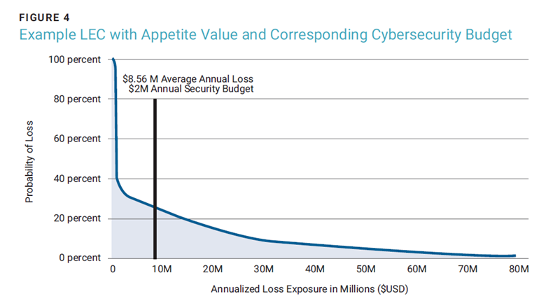
One of the keys to evaluating the suitability of risk appetite is determining how much additional cybersecurity budget would need to be allocated to bring the organization back within risk tolerance. This marginal increase in expenses should be added to the existing cybersecurity budget. The assumption here is that the current amount of spending is resulting in the current amount of risk (figure 4). Therefore, to reduce loss exposure, it is important to adjust spending to account for increased spending on tools, staffing, and processes. One unfortunate artifact of many cybersecurity budgeting practices today is the focus on the acquisition of tools rather than the more important operationalization costs (e.g., the cost of hiring and retaining staff to operate the tools).¹⁵ Thus, it is critical to estimate and include operational tail expenses in budget calculations to continue the proper use of the tools in later years.

Reluctance to increase cybersecurity budgets or to reduce them outright has consequences for the risk appetite threshold setting exercise. Namely, this means that in all likelihood there is a higher threshold of loss than is comfortable for the organization to absorb. This yields three scenarios (figures 5 and 6).

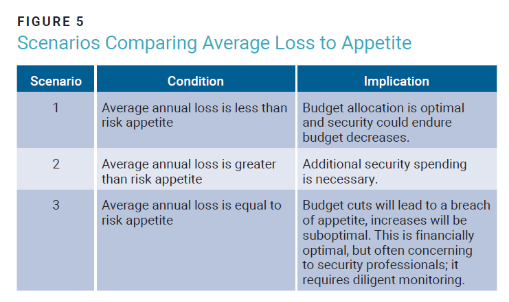
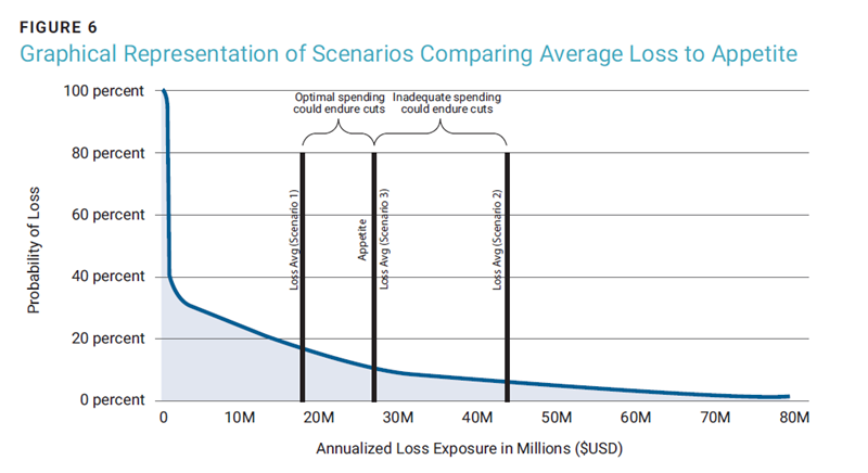
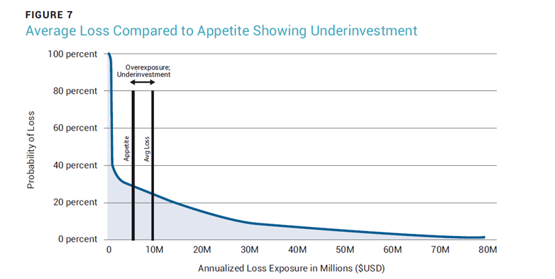
Note here the use of the average or mode value as a comparison point. In terms of having the budget to handle routine, daily security events and incidents, this midpoint value is relevant. Points from higher on the curve are valuable to use when considering risk transfer options later. Referring back to the LEC for the example company, the plot of the average loss shows that there is an underinvestment in cybersecurity leading to an unacceptable loss exposure as shown in figure 7 (average loss of US$8.56 million > US$5 million risk appetite value, or scenario 2 in figure 5). This identifies that there is US$3.56 million in average excess risk liability that must be accounted for.

Like the process for computing the LEC, the curve can be repeatedly simulated with various control states. Next, the relative differences between the control maturity states and their impact on the LEC can be computed. This list of differences essentially shows the organization’s opportunities for improvement and from there, control improvement opportunities can be selected to show how much more security spending is necessary to bring the organization closer to scenario 3.

Figure 8 shows a control domain from NIST CSF: continuous monitoring. The current level of maturity is two, and there are three increased control states shown, corresponding to a standard CMMI scale of 1-5.¹⁶ For each level of increase, there is a corresponding amount of risk reduction, cost to increase the control maturity, and the return on investment (ROI) of that control.

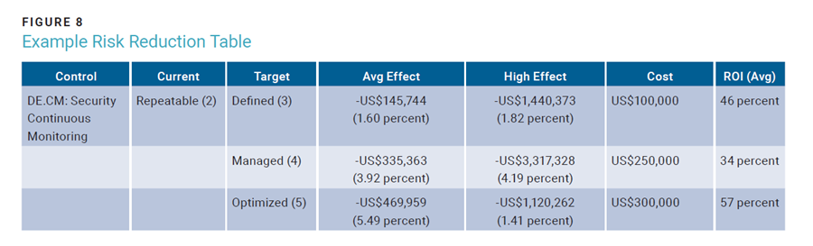
From here, projects can be identified that will reduce risk to within the appetite value. Since risk is measured using the average value, the average effect column can be leveraged to identify the amount of risk reduction. If the project to move continuous monitoring to level five was selected, it would reduce loss exposure to approximately US$3.09M (US$3.56M - US$469,959) and increase the security budget by US$300,000. This process should continue in conjunction with other controls until the expected risk reduction is in line with the risk appetite value, and costs associated with the expense should be added to the security budget for the upcoming year.

Finally, it is worth pointing out that if the organization does not wish to invest in additional controls and keeps the security budget where it is, that implies that the risk appetite threshold was incorrectly selected.

This should initiate a review of the risk appetite and a new threshold should be chosen. Without this feedback loop, an explicit appetite threshold exists, although the organization has not funded the program sufficiently enough to support it, thereby creating an implicit risk appetite. Unvalidated appetite levels do not support good risk governance.

Cyberrisk Transfer

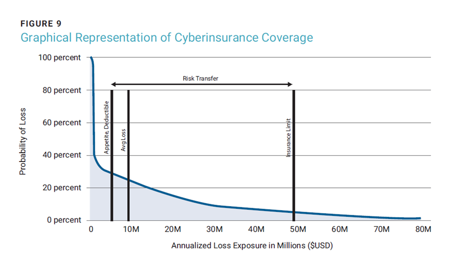
Generally speaking, an organization should not purchase insurance to cover routine occurrences of risk events. This will lead to a high rate of claims and subsequently intolerable increases in premiums. With this in mind, using a higher reference point from the LEC is important for purchasing cyberinsurance. Generally, the coverage window for insurance should cover events that would occur at ten to 100 basis points of revenue or more.

Referring back to the example LEC, the coverage window should start at a value at or higher than the risk appetite. If this kind of deductible is uncomfortable for an organization, it can revisit the appetite threshold setting exercise. But starting at that appetite level and going as high as 100 basis points is a good baseline when shopping for coverage. In the example illustrated in figure 9, coverage begins at US$5 million with a limit of approximately US$50 million. Similarly to the process for setting an appetite threshold, there is a natural emotional and subjective reaction that must be considered based on this analysis. If there is discomfort with the lower or upper levels, they can be adjusted and tested again for suitability with stakeholders.

Risk Resilience Through Capital Allocation

The areas outside the insurance coverage window must be considered for capital allocation. An organization’s ability to absorb losses is a common measure of financial resilience and the use of financial resilience has been applied to cyberrisk.¹⁷ Capital allocation is a formal process for financial services enterprises as regulatory requirements exist to retain capital in case of realized risk. All operational risk sources must have capital allocated to them, and cyber is a recognized type of operational risk.¹⁸ Often organizations conducting capital allocation exercises will retain capital at the 95^th or 99^th percentile. This is known as conditional tail event (CTE) 95 or 99.¹⁹ It means that such organizations will allocate capital to account for loss events assuming they occurred at the 99^th or 95^th percentile (which equates to the 1^st or 5^th percentile in the LEC).

For firms that do not have a formal capital allocation program, it is important to look at the deductible and the risk in excess of insurance limits and account for that. For example, if the deductible is US$5 million, an important question to ask of the chief financial officer is how this would be paid if the organization had to make a claim against the insurance policy this year. Typically, this would be paid either out of the current year’s revenue or ideally out of a reserve fund with money allocated for the risk that may be incurred. Regardless of which option is selected, this decision should be documented and regularly revisited.

Determining the amount of money to consider for capital set aside can be accomplished by analyzing the excess risk, as shown in figure 10. A basic formula can serve as a starting point for this analysis:

Max Loss Exposure - Transferred Risk
- Remediated Risk = Residual Risk

Depending on how conservative an organization wants to be in managing its risk, it can use the value at the 1^st or 5^th percentile as the maximum loss exposure. Subtract the amount of coverage listed on the insurance policy and the risk planned to be remediated from the previous budget exercises. The residual amount would be subject to capital allocation.

Consider 10 bps of revenue as the risk appetite value from the previous example, equating to US$4.49 million in loss exposure, which can be rounded up to $5M. This indicates that the security budget is allocated correctly and no additional risk needs to be bought down by executing additional security programs with a commensurate budget. The value at the 1% point of the LEC was approximately US$80 million. Add to this the cyberinsurance policy with a deductible of US$5 million and a limit of US$50 million. Filling these values into the aforementioned formula yields the following:

US$80M - US$45M - $0 = $35M

This means that there is US$35 million of unmitigated risk that must be accounted for in a capital plan. The deductible of US$5 million should be accounted for in full to ensure that it is available in the likely event the organization must pay out claims. The remaining US$30 million can be allocated using an annualized approach. Given that the insurance runs out at US$50 million, that corresponds to approximately a 6.25% likelihood in the next 12 months. Assuming that value is true for the remaining residual risk (from US$50 million to US$80 million), instead of decreasing in likelihood, there is US$1.875 million (~US$2 million) in annualized risk associated with this extreme loss scenario to contend with. The amount can be allocated, invested, or otherwise earmarked for long-term risk. This is a very basic approach that is suitable for non-financial services enterprises beginning a capital allocation program.

In another example, assume a variance between appetite and average loss increased the security budget. That additional security budget would be accounted for in the remediated risk variable (assuming an additional US$5 million of risk reduction) as follows:

US$80M - US$45M - US$5M = US$30M

This scenario reduces the amount of capital that needs to be accounted for from US$35 million to US$30 million.

Conclusion

There is a growing appetite to govern cybersecurity quantitatively. The NIST CSF 2.0 guidelines increase the importance of governance in a cybersecurity program, highlighting the distinction between higher-level executive roles and day-to-day blocking and tackling of security issues by engineers and analysts. Governing cyberrisk requires an abstraction of daily issues and is best expressed in financial terms by leveraging CRQ. When those assessments have been completed, they must become a part of a regular management review. The work of the executive team should concern itself with three key tasks: budgeting, insurance, and allocation.

Determining the right cybersecurity budget should consider the amount of risk that is comfortable for an organization. Leveraging a materiality assessment can bootstrap this threshold setting. Once the threshold is set, it is straightforward to understand whether more budget is required to align the organization’s appetite. Loss potential above the appetite should be considered with risk transfer strategies (cyberinsurance). Any remaining amount is subject to capital allocation exercises conducted with various degrees of maturity by firms in different industries. Upgrading the maturity of cyberrisk management in the fashion outlined here further brings cybersecurity in line with how enterprises manage other operational risk.

Endnotes

¹ National Institute of Standards and Technology (NIST), NIST Cybersecurity Framework 2.0, USA, 2024, https://nvlpubs.nist.gov/nistpubs/CSWP/NIST.CSWP.29.pdf
² NIST, NIST Cybersecurity Framework 2.0
³ NIST, “Cybersecurity Framework,” USA, https://csrc.nist.gov/Projects/cybersecurity-framework/Filters#/csf/filters
⁴ Freund, J.; “Quantitative Cyber Risk Accelerators,” ISSA Journal, vol. 20, iss. 6, 2022
⁵ Freund, J.; Jones, J.; Measuring and Managing Information Risk: A FAIR Approach, Elsevier/Butterworth-Heinemann, USA, 2014
⁶ Freund, J.; “The Future of IT Risk Management Will Be Quantified,” ISSA Journal, vol. 16, iss. 12, 2018
⁷ The Monte Carlo method leverages random number generation to simulate the uncertainty of future events. For a deeper treatment of this topic and its role in risk management, see Hubbard, D.; The Failure of Risk Management: Why It’s Broken and How to Fix It, John Wiley & Sons, USA, 2009
⁸ Freund, J.; Cyberrisk Quantification, ISACA^®, 2021 
⁹ Freund, J.; “Emotional Cyberrisk Management Decisions,” ISACA^®, 3 January 2024, https://www.isaca.org/resources/news-and-trends/newsletters/atisaca/2024/volume-1/
¹⁰ Freund, J.; Reporting Cybersecurity Risk to the Board of Directors, ISACA^®, 2020; Freund, J.;“Communicating Technology Risk to Nontechnical People: Helping Enterprises Understand Bad Outcomes,” ISACA^® Journal, vol. 3, 2020, https://www.isaca.org/archives
¹¹ Freund, J.; Jorion, N.; “Determining Cyber Materiality in a Post-SEC Cyber Rule World,” ISSA Journal, vol. 21, iss. 9, 2023
¹² Freund; Jorion; “Determining Cyber Materiality”
¹³ Freund; Jorion; “Determining Cyber Materiality”
¹⁴ Freund; Jorion; “Determining Cyber Materiality”
¹⁵ Hill, M.; “Beware the Cost Traps that can Strain Precious Cybersecurity Budgets,” CSO, 16 October 2023, https://www.csoonline.com/article/655295/beware-the-cost-traps-that-can-strain-precious-cybersecurity-budgets.html
¹⁶ Maturity here is used as a proxy for control strength. There are limitations in this approach, but given the ubiquity of maturity assessment approaches, its use here is warranted. Another approach would be to simulate control strength directly.
¹⁷ Google Patents, “Systems and Methods for Assessment of Cyber Resilience,” https://patents.google.com/patent/US20230244794A1/
¹⁸ Sands, P.; Liao, G.; Ma, Y.; Rethinking Operational Risk Capital Requirements, Harvard Business School, 2016, https://www.hbs.edu/behavioral-finance-and-financial-stability/Documents/2016-06%2520Rethinking%2520Operational%2520Risk%2520Capital%2520Requirements.pdf
¹⁹ Freund, J.; “Cybersecurity and Technology Risk,” in Operational Risk Perspectives: Cyber, Big Data, and Emerging Risks, p. 25-46, London: Risk Books, 2016

JACK FREUND | PH.D., CISA, CISM, CRISC, CGEIT, CDPSE

Is the Chief Risk Officer for Kovrr, where he oversees corporate risk and compliance, and strategy and governance of the firm’s cyberrisk products. He is also the co-author of the foundational cyberrisk quantification (CRQ) book using the FAIR standard, which was inducted into the Cybersecurity Canon in 2016. He was named an ISSA Distinguished Fellow, FAIR Institute Fellow, IAPP Fellow of Information Privacy, ISC2 2020 Global Achievement Awardee, and ISACA’s 2018 John W. Lainhart IV Common Body of Knowledge Award recipient. Freund also serves on the board of the ISSA Education Foundation.